An Energy Based Framework for Population Modeling

1. Intro

In the previous post, we proposed a method for eliciting conditional probabilities from a language model, and composing them into joint distributions over arbitrary sets of human characteristics. This gave us a means of capturing the LLM’s priors about the relationships between those characteristics in a form which could serve as a foundation for modeling individuals, and through that the populations they form.

The promise of this approach lies in the breadth of the language model’s latent representation of human behavior. Preferences, beliefs, behavior, and demographics offer a variety of subjects for elicitation, and our previous construction allows us to jointly observe these in order to model relationships for which no corresponding data exists.

Each such cluster of relationships, however, concerns only a local projection of the underlying person we wish to model. How then can we compose these into a more complete representation which fully characterizes our subjects? Likewise, the completed individual, even then, is only one constituent of the population whose behavior we ultimately wish to model. How can we derive a description of the population as a whole from a model of its members in isolation?

In this post, we’ll describe an energy based model which serves to provide a flexible framework for the mechanization of abstraction, via composition, through which both of these quandaries can be addressed. In order to do so, we start by defining the language and notation with which we can discuss and distinguish the abstraction and the abstracted.

2. The Macrostate and the Microstate

We can describe a population through the state of each individual, or through aggregate properties of the population as a whole. To relate these descriptions, let us begin with a complete specification of its members.

Denoting the Microstate

Each agent is a microscopic variable, described by attributes \(A = (A^{(1)}, A^{(2)}, \ldots, A^{(n)})\). Its state is specified by a complete profile:

\[a = (a^{(1)}, a^{(2)}, \ldots, a^{(n)}) \in \mathcal{A}\]

Here \(a^{(r)}\) is the agent’s value for attribute \(A^{(r)}\), and \(\mathcal{A}\) is the space of possible agent profiles.

A realized population is one microstate. For \(N\) agents with profiles \(a_i\), its configuration is

\[x = (a_1, a_2, \ldots, a_N) \in \mathcal{A}^N\]

The configuration space \(\mathcal{A}^N\) contains all possible population configurations. Here \(n\) counts attributes, \(N\) counts agents, and \(i\) indexes agents.

The same configuration can then be described in aggregate, through measurements of its attributes and their relationships. We will refer to these as macroscopic variables. They might describe the share of the population which supports a candidate, for instance, or how income corresponds to vacation frequency. For now, we will focus on marginal proportions, which we can express as proportional shares of attributes among the population.

A macroscopic variable is a function of the configuration. For a fixed attribute \(r\) and category \(k\), the share of agents with that value is

\[m_{rk}(x) = \frac{1}{N} \sum_{i=1}^N \mathbf{1}[a_i^{(r)} = k]\]

The indicator \(\mathbf{1}[\text{condition}]\) equals 1 when the condition holds and 0 otherwise. We use \(m_{rk}(x)\) for a specified single-attribute category share and \(m(x)\) for a general aggregate readout.

The values of our selected macroscopic measurements specify a macrostate. Since many different microstates can yield those same measurements, a macrostate corresponds to a set of compatible configurations.

Distribution over a Population

Our interest in modeling a population lies primarily in its macroscopic properties, though it is through the attributes of individuals and the relationships between them that those properties arise. We therefore need a description which retains this microscopic structure while allowing us to reason about the population in aggregate. While a particular configuration gives us one realization of its measurements, in order to characterize the modeled population more generally, we must consider the underlying distribution from which one population was realized.

We therefore draw inspiration from statistical mechanics, a field concerned with deriving the macroscopic properties of a system from the statistical behavior of its microscopic constituents. It describes a physical system through an ensemble of possible microstates, relating their statistical distribution to the system’s macroscopic properties.

Viewing our population similarly, we can describe aggregate behavior without indexing on the microscopic states of individuals. Doing so requires that we assign probabilities to each possible population configuration.

3. Energy Based Model

The Boltzmann distribution assigns probabilities to microstates based on their total energy, with lower-energies corresponding to higher probabilities. The physical systems for which this was derived have energy in a literal sense, and as such, the meaning of energy in those contexts requires no interpretation. What though is the “energy” of a population?

In the previous post, we proposed a method for approximating the joint probability of an agent’s attribute profile. Using LLM-elicited conditional probabilities to approximate CPDs (conditional probability distributions) for each attribute, we built an offline parameterization of the probability of each attribute \(a^{(r)}\) as a function of its parent attributes \(\pi_r(a^{(r)} \mid a)\). We then composed these individual functions into an auto-regressive factorization of the joint probability across all attributes. Whereas we previously used \(\pi_r\) to indicate the conditional probability function for individual attributes, here we will simply write \(f\) to refer to the joint distribution they factorized

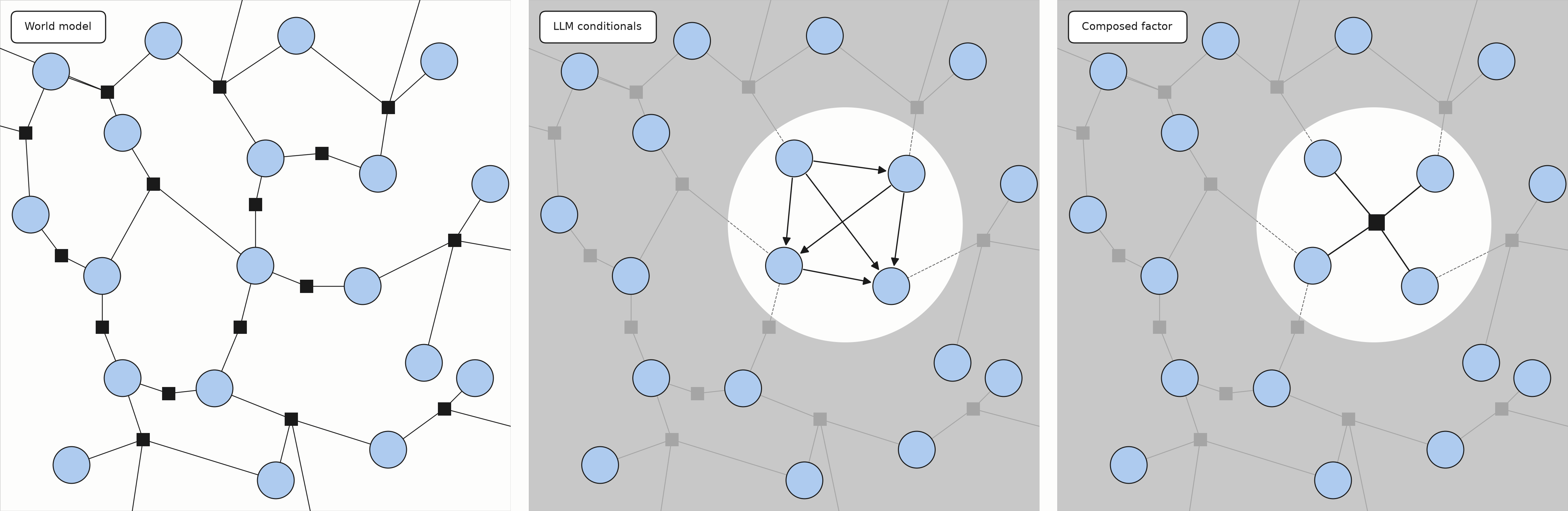
If \(f\) represents the probability for a single agent’s state, we can solve for the energy of a single agent using the same Boltzmann form from earlier. Writing \(\varepsilon(a)\) as the microscopic energy of a single agent, we define the energy as

We will for now assume that the agents within a population are independent of one another. This assumption does not preclude us from later adding interaction effects, but it does allow us to write the microstate’s energy as a sum of its microscopic energies (a skeptical reader can refer to the box below to see that this summation indeed recovers the direct calculation of the population’s probability)

Recovering the Population Level Probability

Since \(f\) is normalized and agents are independent, both population weights and attribute weights sum to 1. This gives us \(Z=1\) for now, so we can simply write:

\[P(x)=e^{-E(x)} \quad \text{and} \quad P(a) = e^{-\varepsilon(a)}\]

By expanding the population energy sum, we can see that:

\[\begin{aligned} e^{ \ -E(x) \ } &= e^{ \ - \sum_{i=1}^{N} \varepsilon(a_i) \ }\\ &= \prod_{i=1}^{N} e^{ \ - \varepsilon(a_i) \ }\\ &= \prod_{i=1}^{N} P(a_i) \end{aligned}\]

Thus recovering the direct computation of the joint probability of a population comprising independently sampled agents

\[P(x) = \prod_{i=1}^{N} P(a_i)\]

Measuring the System

We earlier referred to our macroscopic variables \(m(x)\) as aggregate descriptions of a single microstate. If our system no longer models one particular configuration though, but rather a distribution over all possible populations, our system’s measurements are no longer a direct aggregate calculation on one population. We can adapt by defining our system’s measurements \(\langle m\rangle\) as expectations of the macrovariables over the distribution of microstates.

Configuring the System

In addition to measuring our system, we want a means of controlling its conditions. A simulator which is only capable of modeling a single scenario isn’t of much use after all. Suppose we have a known or desired target value \(C\) for a specific macroscopic readout. Because our measurements are expectations over configurations of the population, satisfying this condition means adjusting our distribution over populations \(P\) such that:

Since we defined our distribution as a function of microstate energies, shifting the distribution is therefore a matter of modifying the energy function such that microstates are reweighted in order to yield an expectation of \(\langle m \rangle = C\).

Recall though that we defined our energy for microstates as a sum of the microscopic energies of its constituents, whose energies in turn were defined as a function of the joint distribution of attributes. It would seem then that satisfying this external condition \(C\) is at odds with preserving the model’s fidelity to the underlying within-agent structure captured by the attribute joint. How then do we reconcile these apparently conflicting requirements of our energy function?

4. Specifying Conditions

When discussing physical systems, we often speak in terms of directly intervening on the macroscopic measurements. While it is sufficient in everyday conversation to say that we “set the temperature” or that we “increased the pressure”, this is, technically speaking, a reductive shorthand. Macroscopic properties are emergent readouts of a system’s state, not independent controls through which the state can be dictated. If we were to take “setting the pressure” literally, it might mean something akin to directly intervening on the particles in a system by e.g. manually accelerating them one by one. Obviously this is not our intended meaning, nor is it in any way feasible.

Instead, controls come in the form of external influences we introduce to the system, and which apply globally to all the microscopics in the system. For example, if we want to modify the magnetization of an object, we can do so by introducing an external field. The particles in the system, each of which is individually acted upon by the field, ultimately settle into a new equilibrium, and the aggregate change across all particles yields a new macroscopic measurement of the object.

Achieving a particular target magnetization then is a matter of finding the field whose influence will act to yield a microstate with the desired aggregate measurements. More precisely, because we model a distribution over microstates, we are solving for a field which shifts the distribution of states such that the resulting expectations of the aggregates, over all possible microstates, match our targets. Rather than interacting with our model by modifying the behavior of individuals (the attribute joint function), we can introduce an external field to our population, which modifies the energy, allowing us to match target conditions while leaving the underlying microscopic model intact.

4.1 Fields

In physics, a field has a very literal interpretation. What does it mean though to subject a population to a “field”? In this case, we will take advantage of the fact that statistical mechanics already models fields in the needed form (as energetic effects on the microscopic variables), and postpone our interpretation, allowing it to eventually follow from, rather than initially motivating, the form.

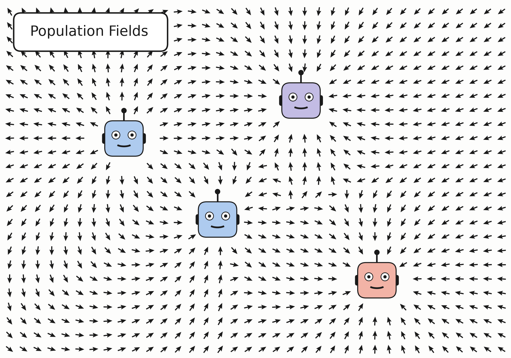
For now, we’ll say that a particular field couples with specific attributes. This is consistent with the physics formulation where, for example, a magnetic field couples with specific microscopic properties (i.e. a particle’s spin, but not its mass). So we’ll write \(h_r\) to indicate a field which couples with the microscopic property (profile attribute) \(r\). When \(h_r\) is applied to the population, we can write the energetic effect it has on each microscopic variable as

where \(\lambda_{rk}\) indicates the field strength for each possible attribute configuration \(k\). In simple terms, this can be understood to mean that, for a microscopic variable with attribute value \(a^{(r)} = k\), the field lowers its microscopic energy by \(\lambda_{rk}\)

We may have multiple fields, each of which couples with its respective microscopic properties. Since fields are additive, we will simply write the combined effect of all fields on a profile’s energy as

We can then update our definition of microscopic energies to include the intrinsic energy \(\varepsilon_0(a) = -\log f(a)\), as well as the effects of all modeled fields

Since agents remain independent of one another, our definition of macroscopic energy as a sum of microscopic energies holds

We can think of that sum of intrinsic energies as the baseline energy \(E_0(x)\). This way, we can write the fields’ effects as contributing to the macroscopic energy as

In this formulation, we can clearly see that we’ve modified our energy, leaving the joint-derived intrinsic energy intact, by modeling the influence of a field on all the individuals within a population

4.2 Fields are exponential tilts of the population distribution

Consider that final sum of the effects of fields applied to each agent in a population. Thinking first about a single field, for a target field on value \(k\) of attribute \(r\), summing over all N agents simply counts how many agents in the population the field applies to

If you recall our definition of a measurement, that summation might look familiar. In fact, it is almost identical in form to \(m_{rk}(x)\), which is simply the share of agents holding an attribute value. We can therefore substitute it in to get the form

Writing \(\boldsymbol{\lambda}\) and \(\mathbf{m}(x)\) for the vectors of field strengths and measurements, respectively, we can rewrite our total energy under the fields as

Writing \(P_\lambda\) for the distribution under the fields, our earlier Boltzmann form gives

So, recalling the baseline population distribution is \(P_0(x) = e^{-E_0(x)}\), we find that the addition of fields is equivalent to an exponential tilt of our initial population distribution!

4.3 Composition vs Causation

In this form, we can finally offer an interpretation of the mechanism we borrowed from physics. A field “acts” on a population by exponentially tilting its distribution, thereby changing its composition by means of reweighting the profiles.

For example, if we were to add a field in order to increase the share of retirees in our population, we would not do so by modeling young people in the population as more likely to retire, but rather by making young people less likely to appear in the population altogether.

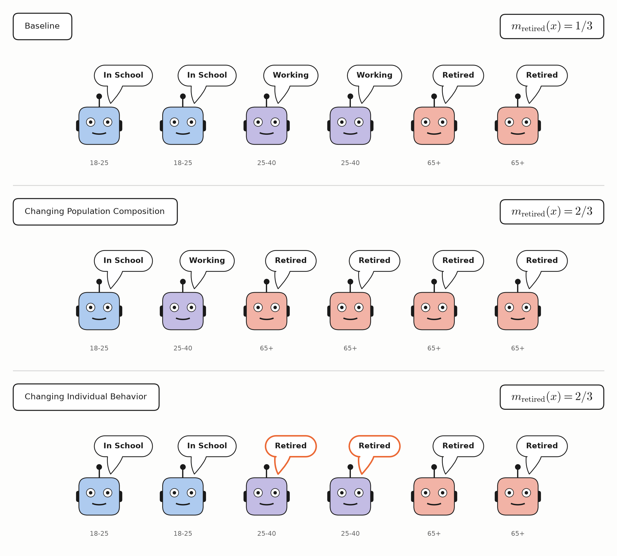
It is clear then that fields can help to resolve the apparent contradiction from earlier, of preserving the coherence of microscopic states, while also allowing us to modify the measurements of their properties in aggregate. The one remaining question then is how to solve for the correct field strength to match specific desired measurements?

4.4 Solving for Field Strengths

The equivalence between external fields and exponential tilts gives us a principled objective for solving for field strengths. Suppose we have a desired macroscopic target \(C_{rk}\) (for instance, an observed share of retirees, or a specific level of policy support). Finding the appropriate field strength means solving for \(\lambda_{rk}\) such that the expectation under the tilted distribution matches our target:

Calibrating this exponential tilt is the classical problem of minimum relative entropy. We can solve for the tilt by minimizing the KL divergence of the tilted distribution from the baseline \(P_0\), subject to the target constraint:

For targets attainable with finite field strengths, the minimizing distribution has our exponential form:

Relative Entropy is Free Energy

In the dimensionless units used above, the free energy associated with the baseline energy \(E_0\) is

\[F_0(P) = \langle E_0 \rangle_P - S(P) = D_{\mathrm{KL}}(P \parallel P_0) + \text{const}\]

Here \(S(P)\) is the entropy of the distribution. Minimizing relative entropy is therefore equivalent to minimizing this free energy subject to the same macroscopic constraints.

We can now draw on the established properties of exponential families to solve for our fields. For targets feasible on the baseline’s support, the minimum-relative-entropy criterion selects a unique population distribution. Each field also provides a predictable direction of adjustment, since increasing its strength while holding the others fixed cannot decrease the corresponding expected measurement.

When we have several conditions to satisfy, we can fit the fields together by minimizing a convex objective whose gradient is proportional to the differences between our expected measurements and their targets. We can therefore use those differences to guide successive adjustments to the field strengths.

5. Incomplete Laws

5.1 The LLM’s World Model

We’ve taken our \(f\) joint function largely for granted in this post. Its construction was the subject of the previous post, which took as a core motivation the idea that we have freedom in choosing which variables to model, since any attribute which can be described as a categorical variable can be included as either a condition or the target question when prompting the LLM.

We can think of the LLM, then, as a source of observations of how attributes relate against the backdrop of its broader latent world. The context of the query determines the scope of our observation, and the resulting joint explicitly describes only the attributes we selected.

Thus far, we’ve spoken in terms of some singular \(f\) and the attributes \(A\) it models. Really, we could have any number of different joint functions for different attribute subsets. We’ll refer more generally, then, to \(f_j(a_{V_j})\) as modeling the joint distribution of some attribute set \(V_j\).

These partial descriptions concern attributes of the same individuals. We therefore need a way to compose them into a single population model, accounting for the relationships each describes and the attributes they share.

5.2 Composing a Factor Graph

Suppose we separately trained several functions \(f_j\) over disjoint sets of attributes \(V_j\). If we were to assume (which we should not generally do) that variables are completely conditionally independent from attributes outside of their set \(V_j\), then our joint functions would be independent. In this case, the distribution over all observed variables so far \(a\) is their product

One thing to keep in mind is that the dimensionality of our \(a\) is no longer static. We are free to elicit new sets of attributes \(V_j\) at any point. But with that aside, our microscopic energy, as the negative log of the probability, is therefore a sum of the energies of each function. Writing \(\varepsilon_j = -\log f_j\), we get

Each joint is locally normalized, meaning their product is as well. So long as our factors are independent, we can compose them by adding their energies. We don’t want to limit ourselves though to only creating compositions of independent factors.

In the previous post, our entire motivation for the autoregressive network was our desire to treat multiple variables as conditionally interdependent parts of a complete, coherent profile. Here, rather than single variables, we have local clusters of attributes, \(V_j\), but we should like to do something similar. Suppose one cluster contains attributes related to a person’s moral philosophy profile, and another cluster contains variables related to political beliefs. We should not assume these are independent

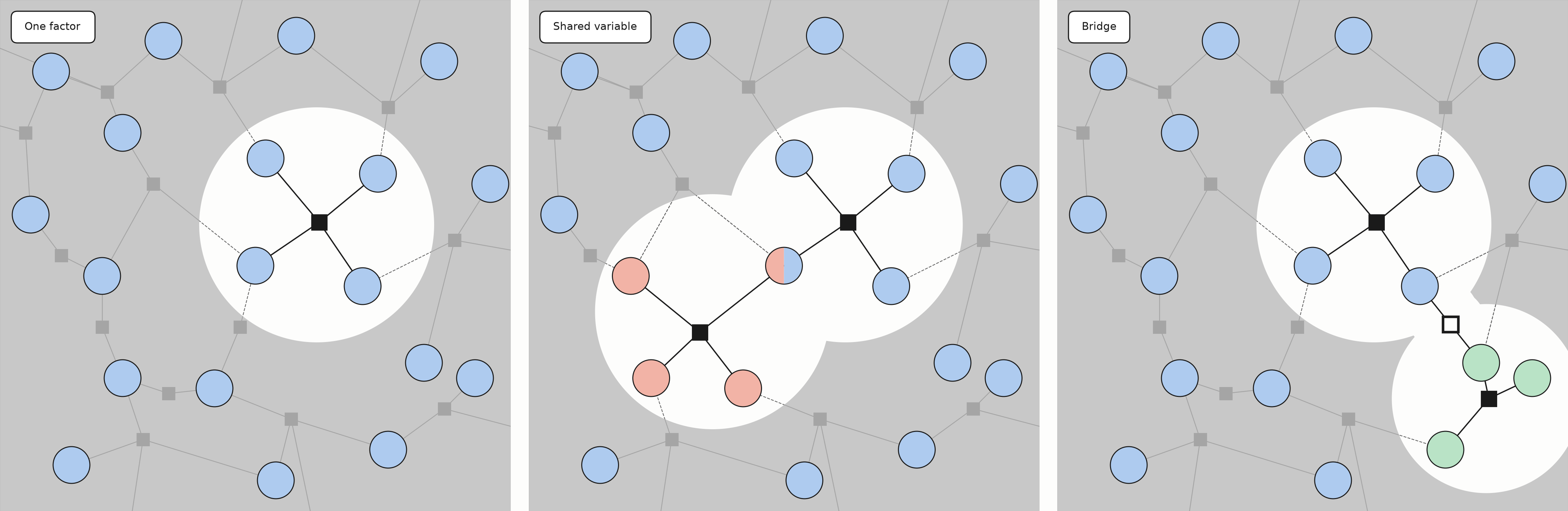
We will consider two means of connecting our local factor clusters then. First, by composing factors which have overlapping variable sets, and then by defining “bridges” connecting existing, disjoint factors.

5.3 Overlapping Variables

Consider the simple case where two sets \(V_1\) and \(V_2\) have a single variable \(r\) in common. Assuming the ideal case, where the marginal probability for \(a^{(r)}\) is the same in both \(f_1\) and \(f_2\), we’ll write \(g(a^{(r)})\) as the marginal probability function (if the marginal differed between \(f_1\) and \(f_2\), we’d have to define a separate \(g\) for each).

Both factors contain this marginal, so combining them would amount to “double counting” it. We therefore divide by the marginal to “remove it” from one of the factors by conditioning on the shared variable.

Under the agreement assumption, the resulting distribution reproduces both joints. We can represent this normalizing operation as a modification to our energy sum by writing \(\varepsilon_r(a^{(r)}) = -\log g(a^{(r)})\), and then subtracting

It is a similar procedure to then add more factors with shared variables, or when factors share multiple variables. By connecting our factors this way, information is able to flow through all variables in the graph through the shared variables connecting the factors.

5.4 Shared Attributes and Bridges

We can include such shared attributes when eliciting our joints, but we can also connect existing models which were originally built with no overlapping attributes. Suppose we want to relate an attribute \(r\) of one to an attribute \(s\) of another. We can elicit a small joint \(f_b\) over those two attributes and use it to connect the larger joints.

Before this connection, the pair has distribution \(g(a^{(r)})\, g(a^{(s)})\), where each marginal is supplied by its respective model. Multiplying by the ratio of the elicited pair distribution to this independent baseline gives

Notice that the second term is equivalent to the shared information between the two variables. We will write its negative log as a new energy \(u_{rs}\) and subtract it from our energy

Technically speaking, there is no distinction between overlapping variables and “bridges”. If we consider our bridge joint to just be an additional factor which shares a variable with each of two existing factors, you’ll see that you’d end up with the same energy, since

We only draw a descriptive distinction so that we can continue to think of our factors as clusters of attributes which collectively describe some greater trait (while bridges can be any collection of related attributes across factors between which we want information to pass). It also allows us to represent our bridge energies in the form typically with which physics represents interacting systems.

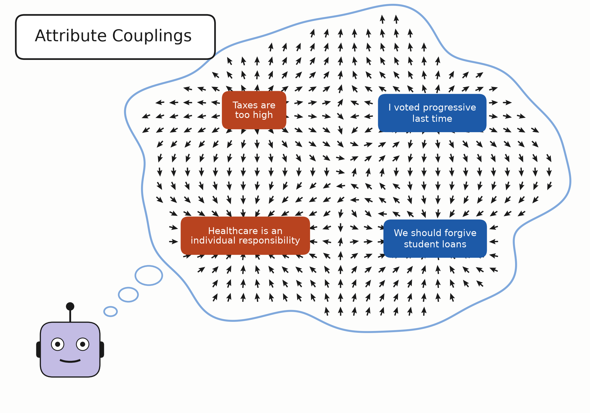
For a collection of initially separate joints and a set \(\mathcal{B}\) of bridged pairs, we can write

In this view, bridges are couplings between attributes. As connections accumulate, a bridge may join attributes already related through other terms, forming a loop. The combined weights then need not sum to one, nor does the resulting distribution reproduce each elicited joint. We can nevertheless retain these connections. Recovering a probability in general requires a normalizing constant \(Z\)

Thus far, we have only been dealing with normalized distributions, and so our \(Z\) was trivial. As we build increasingly rich compositions of factors though, this is no longer necessarily the case. Fortunately, we don’t actually need to compute \(Z\) when we do energy based inference. Notice that, when comparing the probabilities of two profiles, \(Z\) cancels

We can therefore compare profiles without computing the normalizing constant. What remains is to use those comparisons to explore the distribution and compute its measurements.

5.5 Energy Based Inference for Measurements

Gibbs sampling allows the model to explore its possible configurations through a succession of local changes. The relative frequency with which states appear throughout the course of iteration corresponds to their likelihood in the distribution over all microstates. Throughout iteration via Gibbs, our system will tend towards equilibrium, but equilibrium is not a static state. The system’s microscopic configuration will continue to fluctuate around equilibrium. The concept of ergodicity connects this microscopic motion to our macroscopic measurements.

In a physical system, as we’ve discussed, macroscopic properties emerge from the collective configuration of its microscopic constituents. As particles move and collide, that configuration changes, and the macroscopic measurements fluctuate ever so slightly. Just as the configurations fluctuate around some theoretical fixed equilibrium, we can imagine the macroscopic measurements are fluctuating around some fixed value. The measurement we associate with the system then is an average over the fluctuations.

Over a long sampling trajectory, the average of a readout converges to its expectation under the equilibrium distribution. We can therefore estimate that expectation by averaging measurements along the system’s trajectory. Writing \(x_t\) for the population configuration at sampling step \(t\), and \(\mathcal{G}\) for our Gibbs iteration procedure, we estimate our measurements as

Solving for field strengths proceeds as earlier, except that \(\langle m \rangle_\lambda\) is now estimated from the sequence. We iterate, measure, and adjust each field strength in proportion to the remaining error, using a variable step size \(\eta\), repeating this until the estimated measurements match their targets within a chosen tolerance

Adjusting the fields changes the system’s equilibrium distribution. Once the target conditions are matched, we hold the fields fixed and allow the system to equilibrate. Its remaining macroscopic properties can then be measured as averages over the resulting fluctuations.

6. Epilogue

A careful reader may have noticed that, despite describing an ensemble of entire populations, the expected proportions we have been measuring can be obtained from the distribution of a single agent. We have introduced increasingly rich relationships between attributes, though all of these relationships remain within an individual’s profile. The population itself is still a collection of independent draws from that distribution. Have we gone through all this merely to borrow some of the prestige and apparent rigor of statistical mechanics?

Not entirely. Though admittedly, it doesn’t hurt.

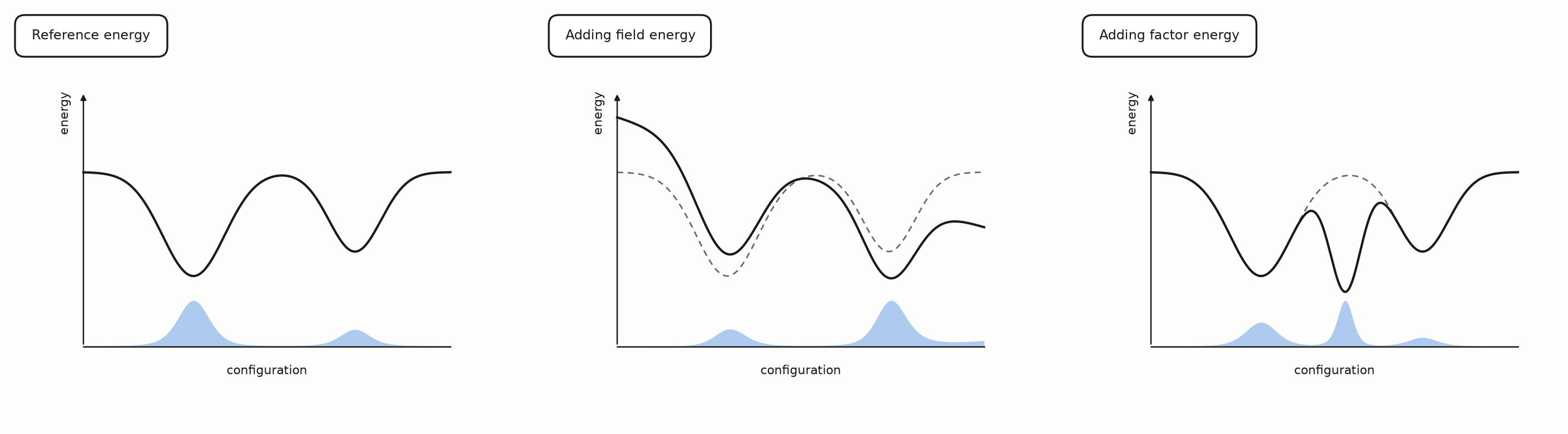
The energy formulation has given us a common means of composing microscopic relationships, imposing macroscopic conditions, and measuring the resulting distribution. Our assumption of independence has also allowed us to postpone a question which becomes difficult to avoid when thinking about populations. What happens when an individual’s state depends on the states of those around them?

Suppose, then, that we allow the energy to depend on relationships between agents as well. For a set \(\mathcal{N}\) of interacting pairs, with \(J(a_i,a_j)\) giving the energetic contribution of each pair, we can write

The probability of a population configuration generally no longer factorizes into independent draws, since changing one profile also changes its contributions to the relationships around it. Those contributions remain available through the energy, allowing us to compare configurations and sample from their distribution as before, now accounting for the connected agents.

This brings us to the question of emergence. A population may exhibit collective patterns which depend on the relationships among its members, so that understanding individuals in isolation is insufficient to explain the population they form. Introducing interactions gives us a way to represent those dependencies, though we still need to understand how they give rise to macroscopic structure. Which relationships sustain a collective pattern, and how might that pattern change as the conditions of the population change? It is this connection between individual dependence and collective behavior that we will turn to next.

Citation

Please cite this work as:

Eigen, Henry. "An Energy Based Framework for Population Modeling". Heigen Thought (Sep 2026). https://henry-eigen.github.io/2026/09/23/energy-based-population-modeling.html

Or use the BibTeX citation:

@article{eigen2026energy,
  title = {An Energy Based Framework for Population Modeling},
  author = {Eigen, Henry},
  journal = {henry-eigen.github.io},
  year = {2026},
  month = {September},
  url = "https://henry-eigen.github.io/2026/09/23/energy-based-population-modeling.html"
}