Distilled-Conditional Bayesian Networks
Summary
In the previous post, we demonstrated that much of the structure of an LLM’s simulated responses for individuals can be captured by a linear, main-effects model, enabling sample-efficient distillation of LLM-estimated conditional probability distributions into lightweight, offline models. In this post, we show how this technique can be applied to build complex simulators of coherent, multi-attribute behaviors. While LLMs cannot reliably generate multi-attribute synthetic individuals in one shot, frequently suffering from mode collapse and failing to capture joint dependencies, they serve as effective suppliers of univariate conditional distributions. We propose the Distilled-Conditional Bayesian Network (DisCo-BN), a framework for building offline simulators by factorizing multi-attribute profiles into a Bayesian network, whose nodes we distill from LLM-elicited conditionals. After a one-time, upfront distillation cost, the resulting network can generate arbitrarily large volumes of coherent synthetic microdata entirely offline. Furthermore, because each node retains an explicit parametric form, the simulator can be calibrated to known ground-truth marginals for empirical grounding, or steered toward target marginals for counterfactual simulation.
1. Response Model vs Simulator
In recent years, LLMs have increasingly been explored as a viable source of behavioral priors where attributes of interest are either not jointly observed, or are unobserved altogether in microdata. The hope is that LLMs capture enough of the latent structure of human behavior and preferences that, when queried with sufficient context on an individual, the LLM can, to a widely debated extent, reason about the individual’s beliefs and intentions, and correspondingly make predictions about the individual’s behaviors.
It has been observed in the literature that LLMs perform much more reliably as suppliers of conditional distributions than they do as sources of samples from joint distributions. That is, they can effectively predict an individual’s response to a single question, given conditioning context on that individual, but when tasked with generating a sequence of responses for an individual, LLMs struggle with coherence within sequences, as well as variance among sequences. This means that the LLM alone can be used as a general response model to independent questions. But it cannot by itself simulate coherent collections of responses for an individual, where the conditional dependencies between responses are non-trivial, or even the primary object of interest. For example, if we predict each response separately:
\[\begin{aligned} a_1 &\sim P(\text{universal healthcare view} \mid \text{individual}), \newline a_2 &\sim P(\text{wealth inequality view} \mid \text{individual}), \newline a_3 &\sim P(\text{voting behavior} \mid \text{individual}) \end{aligned}\]we implicitly assume that an individual’s views on wealth inequality and universal healthcare are completely independent of how they vote. Such an assumption undermines the utility of a simulator, both for generating realistic individual profiles and for conducting population-level analysis. In analysis, we want to understand how beliefs and behaviors cluster together, or how a shift in sentiment on one topic would affect support for another. To capture these relationships, we must be able to simulate sequences of attributes that are coherent over the joint conditional distribution:
\[(a_1, a_2, a_3) \sim P(\text{healthcare view}, \text{inequality view}, \text{voting} \mid \text{individual})\]Autoregressive Factorization
We’ve already established that LLMs should not be directly queried for joint distributions, but this does not mean that they are altogether unable to supply them. Using the chain rule of probability, we can factorize the desired joint conditional (which the LLM cannot supply) into a series of univariate conditionals (which it can supply). Then, by eliciting responses sequentially, conditioning each on those generated before it, we can autoregressively create sequences which, although elicited one at a time, are coherent over their joint distribution.
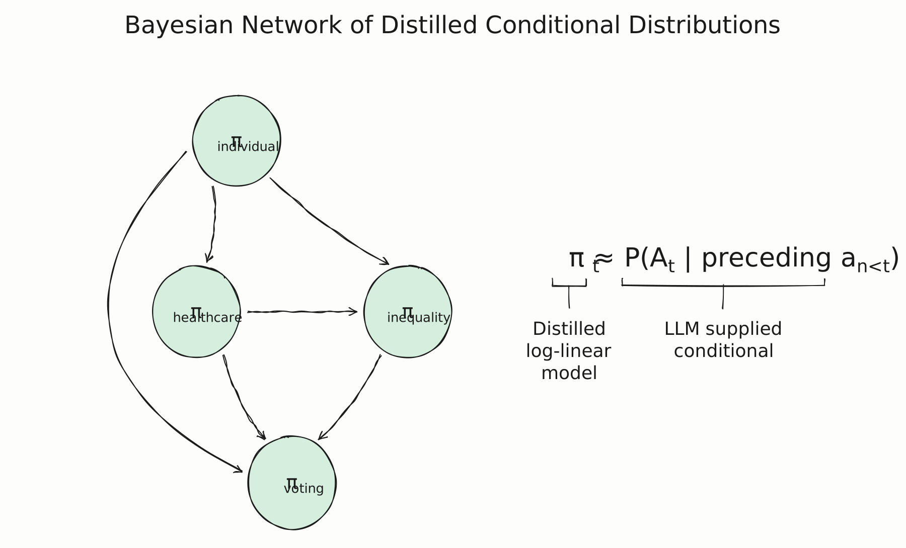
\[\begin{aligned} a_1 \sim P(\text{universal healthcare} &\mid \text{individual}), \newline a_2 \sim P(\text{wealth inequality} &\mid \text{individual}, \text{healthcare}), \newline a_3 \sim P(\text{voting behavior} &\mid \text{individual}, \text{healthcare}, \text{inequality}) \end{aligned}\]This factorization is the basis of a Bayesian network, where the conditional distribution for each attribute is represented as a node, and the preceding attributes upon which a node is conditioned are connected by edges. Since this autoregressive generation amounts to sampling from the joint conditional, we get coherent sequences of responses. And since we randomly sample according to the distribution at each node, we preserve the full variance of the population, thus avoiding the mode collapse faced when eliciting sequences directly from the LLM.
Building a Bayesian Network out of Distilled Conditionals
Querying a live LLM sequentially for each generated individual would render large-scale simulation prohibitively expensive. This is a problem we partially addressed in the previous post, where we showed that we can distill an LLM’s conditional distributions into offline log-linear models. In this post, we demonstrate how this same distillation approach can be used to construct the nodes of our Bayesian network. We query the LLM during an initial setup phase to estimate each node, and then run the simulation entirely offline. Having explicit parametric models at each node also gives us capabilities that an LLM alone cannot provide, including better calibration, increased interpretability, and the ability to construct counterfactuals which diverge from the LLM’s world model.
2. Factorization and Generation
In order to simulate a coherent collection of attributes for an individual (an individual’s response to a question being an example of an attribute), we factorize the joint distribution of attributes as a Bayesian network. That is, we define a directed graph where each node corresponds to a single attribute \(A_t\), and directed edges indicate conditioning relationships between nodes. In the most general case, making no assumptions of independence between attributes, we consider each node’s parent set to contain all preceding attributes. Given initial seed attributes \(A_c\), the network then factorizes the joint conditional distribution as:
\[P(A_1, A_2, \ldots, A_n \mid A_c) = \prod_{t=1}^n P(A_t \mid A_c, A_1, \ldots, A_{t-1})\]This graphical representation does require assigning a topological ordering to the nodes in the graph, and therefore to their corresponding attributes. Unlike text sequences or time-series data, our various demographic and behavioral attributes have no intrinsic order. Any ordering is an equally valid factorization under the chain rule, rendering order assignment a practical consideration. Since it determines which conditionals are elicited from the LLM, it is possible that some orderings will yield prompts with more stable responses from the LLM. We will consider this choice to be an implementation detail beyond the scope of this post. Likewise, our assumption of a fully connected network is not a requirement of our method generally, but we leave pruning decisions to implementation.
Bayesian networks can be used as generative models through forward sampling. This process involves traversing the graph, and instantiating a value at each node by sampling its conditional distribution using all previously instantiated values for conditioning. Sampling is initiated by specifying some seeded context values \(A_c\) for the root nodes.
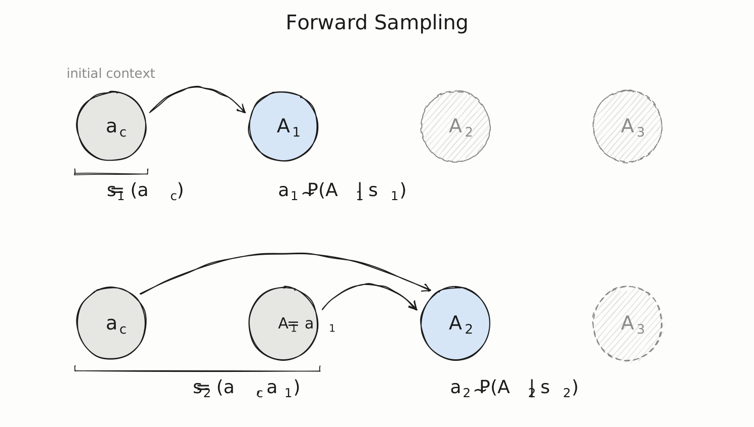
We frame this autoregressive generation as a sequential decision process where, at step \(t\), the state \(s_t\) contains the sequence of all values instantiated so far (including the initial \(a_c\)):
\[s_t = (a_c, a_1, \ldots, a_{t-1}) \quad \rightarrow \quad a_t \sim P(A_t \mid s_t) \quad \rightarrow \quad s_{t+1} = (a_c, a_1, \ldots, a_{t-1}, a_t)\]3. Learning the Network
When modeling Bayesian networks, it is standard practice to express each node’s conditional probability distribution as a parameterized function, and to jointly fit all functions (one per node) using a shared corpus of fully observed data. We will adopt the former approach, defining a conditional probability function \(\pi_t\) for each node \(t\), such that
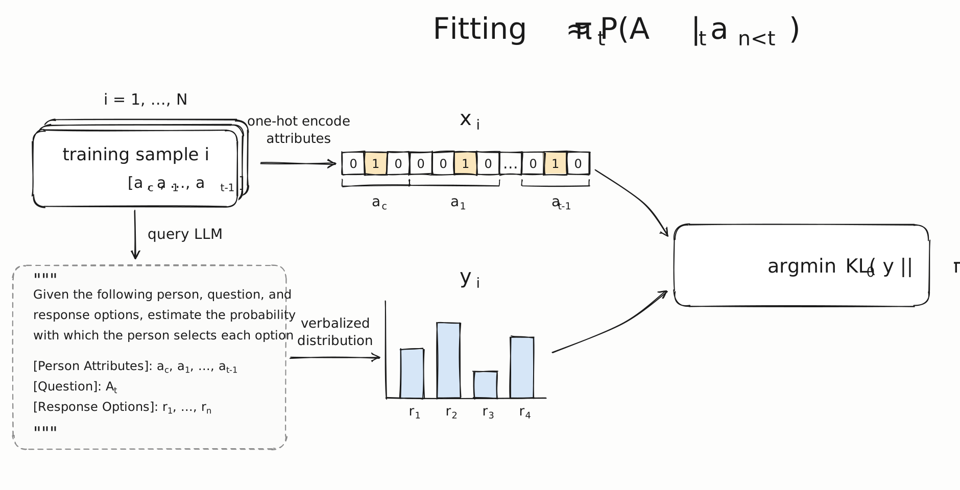
\[\pi_t(\cdot \mid a_c, a_1, \ldots, a_{t-1}) \approx P(A_t \mid A_c=a_c, A_1=a_1, \ldots, A_{t-1}=a_{t-1})\]As for the latter however, the non-existence of such fully observed data is the entire premise of this post. What is instead available to us is the LLM, which can provide approximations of conditional probabilities given conditioning attributes we supply as context. We therefore treat parameter estimation of our functions as a knowledge distillation problem, using the LLM as a teacher model, rather than an empirical data-fitting problem.
Unlike typical estimation, where the same dataset of joint observations serves the entire network, each of our LLM queries supplies values for one specific set of conditioning attributes and returns a distribution for one specific attribute, so data elicited to train one node cannot be recycled to train another. Our distillation loop therefore involves separately eliciting data for the fitting of each conditional function.
For every node \(t\), we generate a batch of training inputs \(s_t^{(i)}\), each comprising one value for each of the node’s conditioning attributes. For each input, we then elicit from the LLM a probability distribution over possible values for the node’s attribute, and treat this as the training target \(y^{(i)}\). We use these training inputs and targets to learn our function parameters \(\theta_t\) by minimizing the forward KL divergence from the elicited distributions to our model’s distributions.
At a high level, learning our full Bayesian network appears to be a simple matter of repeating this distillation process for every node in the graph. In practice however, translating this abstract single-node loss into an end-to-end generative simulator is not quite so straightforward. Because the LLM is an unconstrained oracle, we could theoretically prompt it with arbitrary combinations of conditioning attributes. But with a finite query budget, and an imperfectly fitted model, we want to train \(\pi_t\) on the specific parent configurations, drawn from \(P(A_c, A_1, \ldots, A_{t-1})\), that the simulator will actually encounter during generation. This creates an apparent chicken-and-egg problem, in that we need samples from the joint distribution to train the conditional functions, but we are learning the conditional functions precisely to define that joint distribution.
The combinatorial state space \(\mathcal{A}_c \times \mathcal{A}_1 \times \cdots \times \mathcal{A}_{t-1}\) grows exponentially with each additional attribute. The vast majority of this product space consists of nonsensical or vanishingly rare combinations. Sampling arbitrary combinations across this space exposes us to the classic off-policy covariate shift problem in imitation learning. When a student policy is trained on an off-policy distribution of states, rather than the distribution generated by its own sequential rollout, small estimation errors compound quadratically along the rollout trajectory.
Compounding this issue is the nature of the oracle itself. While an LLM will obligingly return a probability distribution for any prompt we hand it, we cannot expect grounded or coherent conditionals on nonsensical, off-manifold profiles that have no basis in human reality. Fitting our student models on these phantom states distorts the learned parameters in the realistic regions where the model actually needs to operate.
Sequential bootstrapping
We therefore use on-policy sequential bootstrapping, which directly mirrors the Forward Training algorithm in imitation learning. To construct the network, we seed a training population by sampling context attributes \(A_c \sim P(A_c)\). For each subsequent attribute node \(t\), we treat the learned prefix \((\pi_1, \dots, \pi_{t-1})\) as an active, self-contained Bayesian network and use closed-loop forward sampling to generate our training states:
\[s_t^{(i)} \sim P_{\pi_{1:t-1}}(s_t)\]We query the LLM oracle exclusively on these student-generated states, fit \(\pi_t\) by minimizing the empirical forward KL, and sample \(a_t \sim \pi_t\) to form the states for node \(t+1\). Every node is thus trained strictly on-policy with respect to the preceding prefix, eliminating rollout distribution mismatch between the states used for training, and the states expected in deployment.
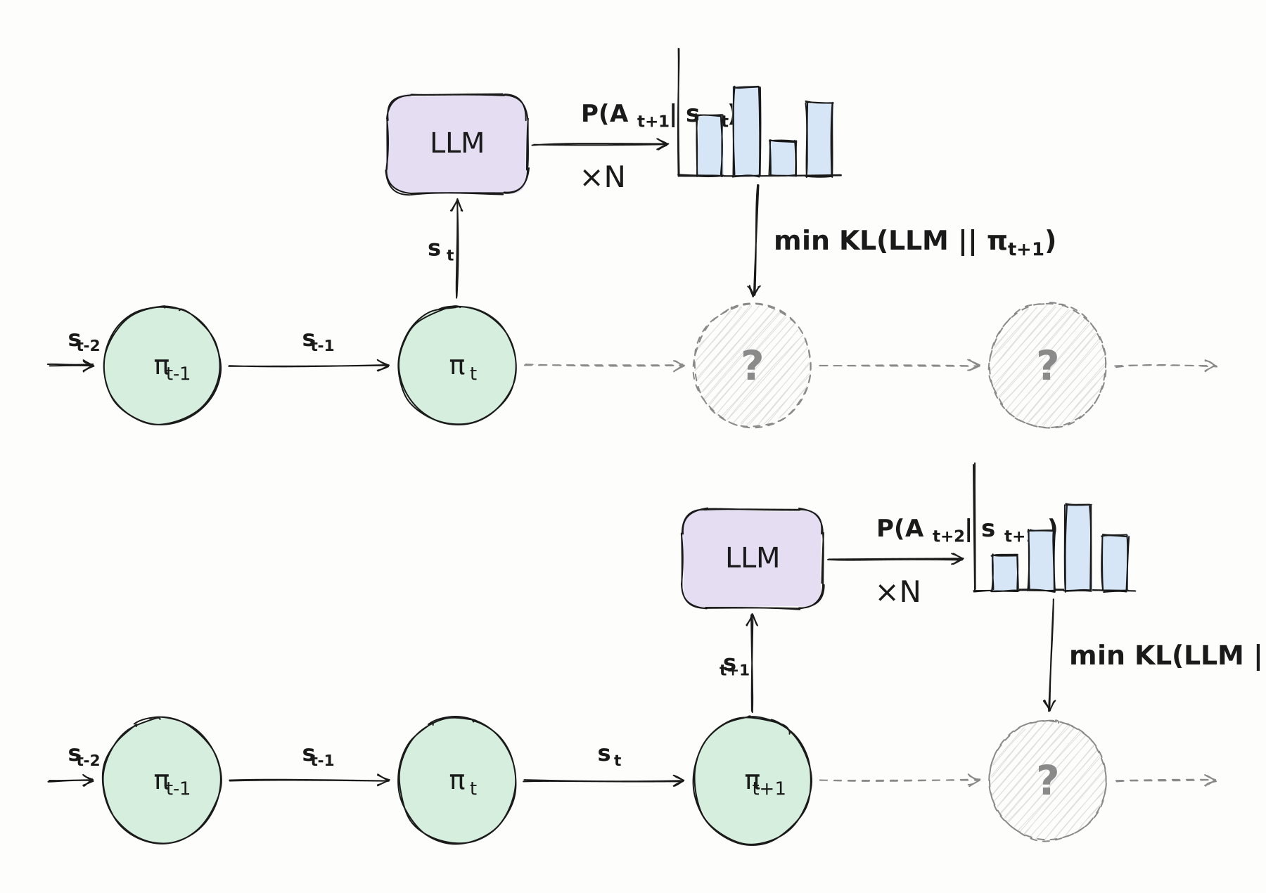
Crucially, unlike standard imitation learning where an expert provides only a single discrete demonstration action (or scalar reward), our oracle returns the full categorical probability distribution over all response options. Minimizing forward KL divergence against this soft target forces the student to match the full variance, entropy, and relative probabilities of the teacher’s conditional distribution, rather than collapsing to a single mode.
4. A demonstration of the network
To demonstrate this process, we will create a response model for a collection of questions which no survey asks collectively. We will take the topical issue of public sentiment on AI as the subject of our model. We start by hand crafting 16 questions about AI, economic policy, and general public opinion, the categorical responses to which will be the attributes for our agents. Three examples of the questions:
-
Thinking about the U.S. over the next 20 years, do you think that artificial intelligence (AI) will lead to more jobs, fewer jobs, or will not make much difference?
Response options: “More jobs”, “Will not make much difference”, “Fewer jobs”, “Not sure”
-
Thinking about the use of artificial intelligence (AI) in the United States, are you more concerned that the U.S. government will go too far regulating its use or not go far enough regulating its use?
Response options: “Go too far regulating its use”, “Not go far enough regulating its use”, “Not sure”
-
Thinking about the U.S. over the next 20 years, what impact do you think artificial intelligence (AI) will have on medical care?
Response options: “Very or somewhat positive”, “Equally positive and negative”, “Somewhat or very negative”, “Not sure”
The node functions
Our DisCo-BN method in general does not prescribe any specific architecture for the node functions. For our experiments here, we used a simple log-linear model at each node, where a single parameter from each input attribute, selected by that attribute’s value, adds to create a logit for each output option. The logits are then passed through a softmax to obtain the probabilities for each output. Using \(\mathbf{x}_j\) as the one-hot encoding of input attribute \(a_j\):
\[z_k = b_k + \mathbf{x}_1^\top \mathbf{w}_{1,k} + \mathbf{x}_2^\top \mathbf{w}_{2,k} + \ldots + \mathbf{x}_n^\top \mathbf{w}_{n,k} \qquad p(k) = \frac{\exp [z_k]}{\sum_{k'} \exp [z_{k'}]}\]We found that this simple model was sufficient to learn the LLM’s conditionals well, and its light parameterization provides us with sample efficiency and desirable optimization properties. There is no reason more complex functions couldn’t be used instead if, for example, we wanted to integrate interaction terms or add hidden layers. We’ll leave comparisons between functions for another time.
Training the functions
We trained the nodes in sequence as described in Section 3, forward sampling the training states for each node from the nodes already fitted before it. Because the LLM is our source for training data, we can elicit as many samples as we desire. That said, each additional sample adds to our inference costs, so we want to elicit no more than is needed to converge on a fit. Our selected logit model is parameter light, and sample efficient. For a given node function, its parameter count for each output logit is one for each level of each input attribute. After fixing reference levels for inputs and outputs, a node with \(K\) response options and input attributes with \(L_j\) levels has a free-parameter count of
\[p = (K - 1)\left(1 + \sum_j (L_j - 1)\right)\]Across all nodes this comes to 1,228 free parameters. We trained each node on multiples of its own \(p\), showing in the table below the average performance across node functions for increasing multiples of \(p\). Performance here is a measurement of each function’s accuracy against held-out LLM samples. We found that the majority of the fit was achieved by \(2p\), but doesn’t fully flatten until a few multiples beyond that. At \(4p\), the budget we used for the final network, the full training set cost around $15 in LLM inference (not including evaluation samples).
| Average across nodes | 1p | 2p | 3p | 4p |
|---|---|---|---|---|
| KL skill (higher is better) | 79.30% | 89.15% | 90.32% | 90.98% |
| Mean TVD (lower is better) | 5.33% | 4.07% | 3.82% | 3.69% |
| Mean Spearman coefficient (higher is better) | 0.868 | 0.913 | 0.922 | 0.925 |
Of the three metrics, we care most about the Spearman coefficient, which measures whether our model agrees with the LLM about which profiles are more or less inclined toward each answer. The conditional structure matters because it determines which other views accompany an opinion we change in a scenario. Suppose people expecting AI job losses are more likely to support an AI dividend. Giving greater weight to profiles expecting job losses will then also tend to increase dividend support. A model that reverses this association could match the same population totals yet predict the opposite scenario response.
Performance varied across questions, but showed no clear relationship to where a question sat in the ordering. An early node was not inherently fitted better than a late one.
| Per node | KL skill | Mean TVD | Mean Spearman |
|---|---|---|---|
| Economic inequality | 91.55% | 4.00% | 0.897 |
| Government living-standard responsibility | 96.47% | 2.93% | 0.955 |
| Business regulation | 97.21% | 3.14% | 0.982 |
| Corporate taxes | 95.26% | 3.75% | 0.975 |
| … | … | … | … |
| Guaranteed-income support | 98.10% | 2.32% | 0.976 |
| AI-dividend support | 96.77% | 3.72% | 0.927 |
| Public-AI support | 92.19% | 4.68% | 0.906 |
| AI-ownership policy support | 91.25% | 4.55% | 0.905 |
Inference
Thus far, we’ve only discussed forward prediction, where the autoregressive ordering specifies how we construct and sample the joint. Once trained however, we are not restricted to conditioning predictions on just the values accepted by a node’s function. The product of the node functions defines a full joint distribution over the attributes, and like any Bayesian network, it allows for posterior inference, where we condition on any subset of attributes and query any other, regardless of where they sit in the ordering. The ordering was needed to define and train the joint, however it places no restriction on how we query it once trained.
For any single unobserved attribute \(A_i\), we can calculate its full conditional given all other attributes \(A_{-i}\), whether they precede or succeed \(A_i\) in the network. To do so, we score the probability of the full response profile under each candidate value, and then normalize over all candidates (since the probabilities across all candidates must sum to 1):
\[\pi_\theta(A_i=k \mid a_{-i}, a_c) = \frac{\pi_\theta(k, a_{-i} \mid a_c)}{\sum_{k'}\pi_\theta(k', a_{-i}\mid a_c)}.\]In order to evaluate how well our network performs this order-agnostic inference, we used forward sampling to generate a representative population of full profiles, and randomly selected one attribute from each to be our held-out \(A_i\). We then passed all other attributes \(a_{-i}\) to the LLM, eliciting distributions for the held-out attribute, and evaluated our model against those targets much as we did for training evaluation.
| Mean across nodes | KL skill | Mean TVD | Mean Spearman |
|---|---|---|---|
| Forward conditionals | 90.98% | 3.69% | 0.925 |
| Arbitrary conditionals | 81.99% | 6.20% | 0.912 |
KL skill and mean TVD both degraded relative to the forward conditionals. We are not so concerned about this though, since our Spearman coefficient, the metric we are most concerned with, shifted little. Our inference retains strong agreement with the LLM about which profiles are more likely to give which answers, despite a moderate degradation in absolute magnitudes.
A concrete example
Suppose we only have values for a subset of attributes. We can fix them, and then marginalize over the rest. Consider the example in the figure below. We selected several attributes for which we fixed values, giving two profiles that differ only on those attributes, and then sampled the remaining attributes from the network conditioned on those values. From these samples we can inspect the marginal distribution each profile gives on any of the remaining questions.
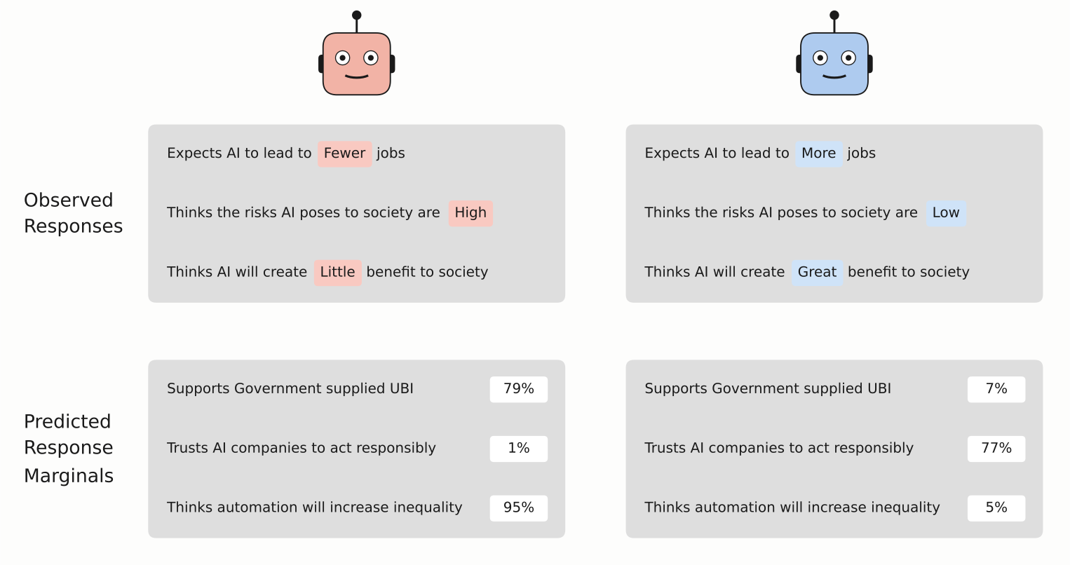
The numbers in the figure are the real outputs of our network. The network models a collection of hand-crafted questions which no dataset we found jointly observes, so all conditional structure among the questions came solely from the LLM. This means that we can’t evaluate the accuracy of the responses (although the relationships seem intuitively reasonable), but it also means the conditional structure wasn’t memorized. Keep in mind too that this small, offline network cost only $15 worth of LLM inference to train. Pretty neat.
Citation
Please cite this work as:
Eigen, Henry. "Distilled-Conditional Bayesian Networks". Heigen Thought (Aug 2026). https://henry-eigen.github.io/2026/08/19/distilled-conditional-bayesian-networks.html
Or use the BibTeX citation:
@article{eigen2026disco,
  title = {Distilled-Conditional Bayesian Networks},
  author = {Eigen, Henry},
  journal = {henry-eigen.github.io},
  year = {2026},
  month = {August},
  url = "https://henry-eigen.github.io/2026/08/19/distilled-conditional-bayesian-networks.html"
}