Simulating the Effects of Fields on Simulated Agents

Overview

In previous posts, we proposed a method for modeling the joint distribution of responses within LLM-simulated agents. We elicited, from an LLM, conditional probabilities corresponding to how a described agent would answer each new question, given its responses to previous questions. By learning the LLM’s mappings from observed responses to the likelihoods of yet-unobserved responses, we distilled the LLM’s model for each conditional probability distribution into a compact, offline representation. By composing these distillations autoregressively, we obtained a network representing a joint distribution over complete response profiles.

We previously demonstrated that our network could then be used to generate populations of coherent, representative agents by capturing the dependencies among the response attributes within each agent. But the resulting population was static, with no mechanism by which to update agents over time in response to between-agent social interactions or other modeled external influences.

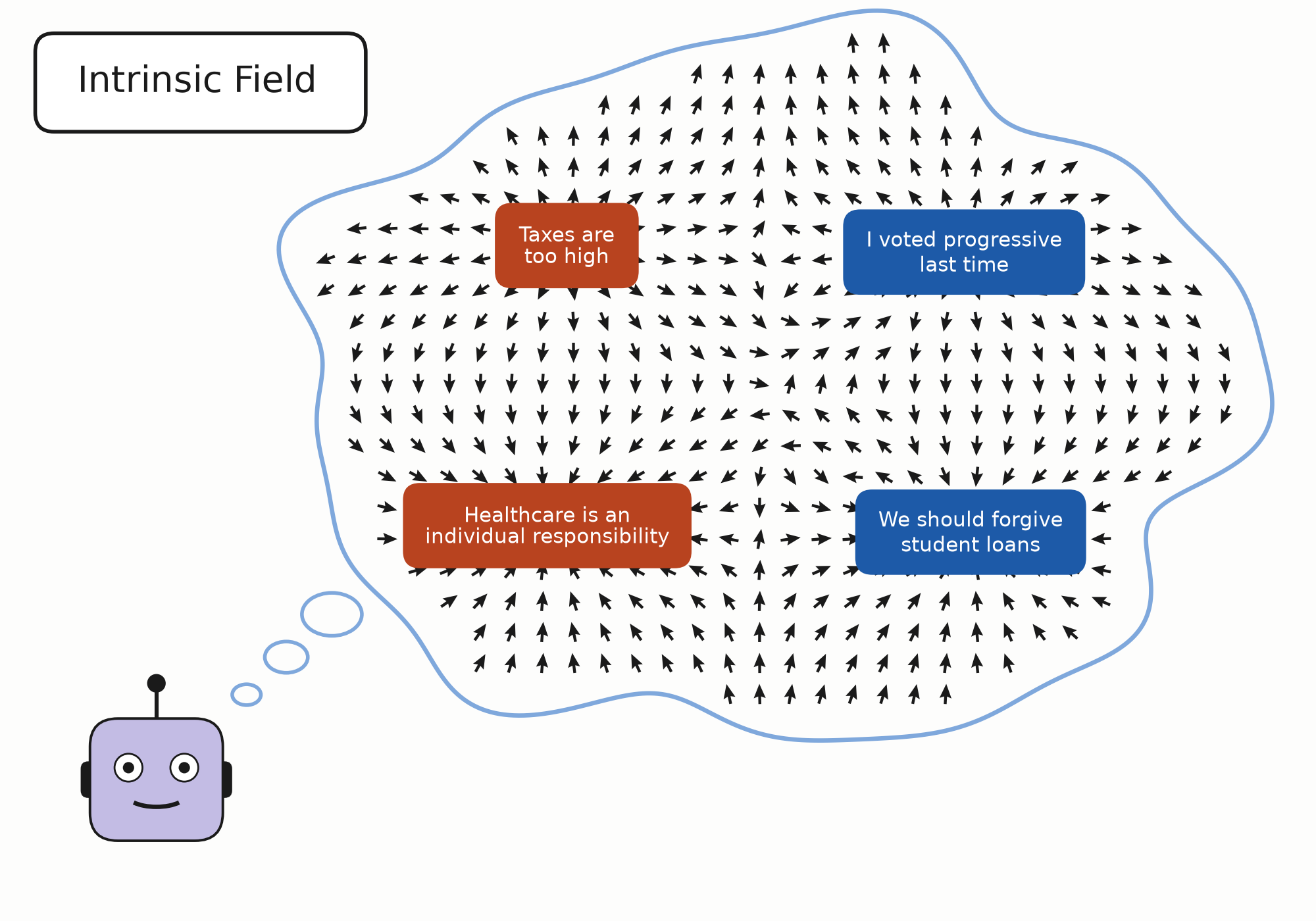
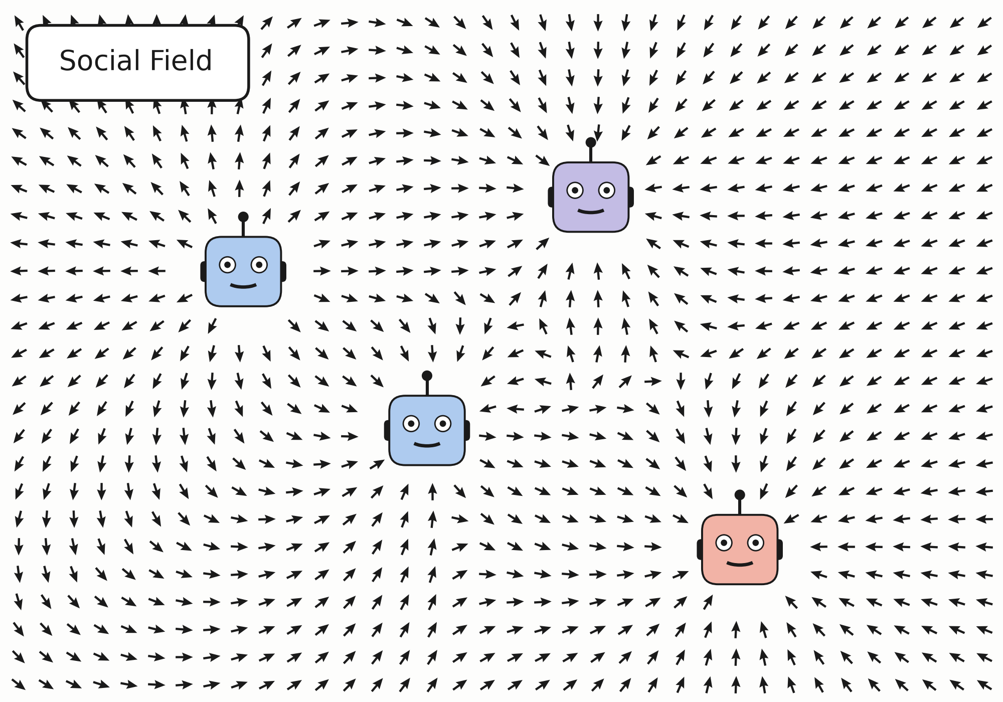
In this post, we will demonstrate a previously unexplored capacity of our network by defining such a mechanism. By reinterpreting our learned joint distribution as a baseline energy surface, and modeling influences external to an agent as fields, we can derive an update operator for agents, through which our population can change dynamically over time.

We begin with a brief recap of our joint network, DisCo-BN. Readers familiar with the method can skip directly to Section 1

Recap

Distilling Conditionals

Suppose agent profiles are composed of categorical response variables \(A = (A_1,\ \ldots,\ A_n)\). A particular agent has a realized profile \(a = (a_1,\ \ldots,\ a_n)\), where \(A_i=a_i\) means the agent gave response \(a_i\) for question \(i\). We can provide an LLM a description of the agent’s earlier responses and relevant context, and elicit in turn a conditional distribution over a yet-unobserved response:

By repeating this elicitation for a variety of agent profiles, we can build a training dataset of conditional distribution targets with which to fit an offline model \(\pi_t\):

Composing Distilled Conditionals into a Bayesian Network

While univariate conditionals can be reliably elicited from the LLM, various methods for directly eliciting a joint conditional over multiple unknown attributes are either unreliable, or infeasible at scale:

Rather than trying to elicit the joint from the LLM directly, we factorize the desired joint probability as a product of univariate conditionals elicited from the LLM. DisCo-BN expresses this factorization as a Bayesian network, and parameterizes each node \(t\) with \(\pi_t\).

Nodes are trained sequentially using an on-policy distillation loop where, for each node, LLM targets are elicited on partial profiles generated by the already-fit, upstream portion of the network. The fitted conditionals then compose into a normalized joint over complete profiles:

For the full elicitation and training methodology, see our DisCo-BN post

1. A simple model of social interactions

We are interested in a mechanism which allows us to model the ongoing effects of external influences on our agents, so that we can simulate a dynamic population which evolves over time. As a starting point, we consider a simple model of social influence proposed in the recent paper Physics of Agents.

The paper derives a local update function for agents from an Ising energy model, where an agent’s predisposition towards a state combines with social influence from its neighbors in order to yield its future state. For an agent \(i\) with currently held binary opinion \(s_i\in\{-1,+1\},\) the probability of its post-update state \(s_i^{\mathrm{next}}\) is given by:

Here, \(g_i\) is the agent’s intrinsic field, defined as its baseline predisposition towards one state as opposed to the other, absent any external influence. Because the modeled opinion is binary, this single contrast completely describes the relative intrinsic support for its two possible states:

In addition to the intrinsic field, an agent’s update includes a social field, represented by the second term in the sigmoid. The signed connection \(J_{ij}\) determines how agent \(j\)’s opinion bears on agent \(i\), while \(\beta\) controls the strength of that influence. The two fields combine additively in log-odds space.

2. Generalizing the local update

While we take this as our starting point, the paper’s update function makes two assumptions about modeled agents which we do not want to carry over to our application.

1. It assumes that agents hold a single opinion, or at least that individual opinions are independent of one another. This is in contrast to our use-case, where the entire motivation for DisCo-BN is to model agents composed of multiple, interdependent attributes.
2. It assumes that opinion attributes are binary, whereas our model supports categorical attributes with arbitrary numbers of states.

To adapt their update function for our purposes then, we first propose a generalized form which allows agents to possess multiple, categorical attributes.

Potts Model

To extend the paper’s binary Ising formulation, we draw on the standard Potts generalization from binary to categorical states, and apply that categorical-state perspective to agent profiles containing multiple attributes. Whereas the original formulation assigns energies to the two states of a single binary attribute, we treat an agent’s complete categorical profile as its state.

Suppose agent profiles generally contain values for attributes \(A = (A_1,\ A_2,\ \ldots,\ A_n)\). So a given agent’s profile is \(a = (a_1,\ a_2,\ \ldots,\ a_n) \in\mathcal A\), where \(a_r\) is the agent’s value for attribute \(A_r\). Treating an agent’s full profile as its state then, we assign each profile an intrinsic energy:

Updating the Intrinsic Field

In the single-attribute, binary case, an agent has one of only two states. A two-state intrinsic distribution has only one independent contrast, making it easy to represent \(g\) as a single scalar:

In the original paper’s single-attribute setting, there were no other within-agent attributes on which intrinsic support could depend. In our multi-attribute setting though, the marginal probability \(P(A_r=k)\) would average over the configurations of the remaining attributes, thereby ignoring how coherently \(A_r=k\) fits with the rest of a particular agent’s profile. We therefore condition the agent’s intrinsic support for \(A_r=k\) on the rest of its attributes, denoted \(A_{-r} := (A_s)_{s \neq r}\), using the conditional probability:

For the purposes of this post, we’ll model incremental changes by updating one attribute at a time while retaining the complete profile as the agent’s state. We write \(a_{r\leftarrow k}\) for the profile obtained by setting \(A_r=k\) and leaving the remaining attributes unchanged. Because of our simplifying assumption that \(a_{-r}\) is held fixed during an update to \(A_r\), we normalize only over the candidate profiles \(a_{r\leftarrow k}\) :

For an attribute \(A_r\) with \(K\) possible states, the conditional distribution has \(K-1\) independent log-odds contrasts, one for each non-reference option \(k\) against a common reference option \(k'\). Because the intrinsic field does not reduce to a single scalar in our case, we will not adopt the notation \(g\), and instead use its log-odds definition directly:

Updating the Social Field

To extend the social field to the categorical case, we can simply use the standard Potts interaction. For focal agent \(i\) with neighbor set \(\mathcal N_i\), we assign candidate state \(A_r = k\) the social score:

As in the original formulation, this simply selects the terms \(J_{i, j}\) for which neighbor \(j\text{'s}\) value for \(A_r\) matches candidate \(k\) for agent \(i\), with \(\beta_r\) determining the interaction strength for attribute \(A_r\). We can sum these attribute-wise scores in order to define a social field over complete profiles:

Under our simplifying assumption, that one attribute is updated at a time, the social contributions of all unchanged attributes cancel out when comparing two candidate values for \(a_{r\leftarrow k}\)

3. Bringing it all together

Now that we have generalized the form of the update function to support agent profiles composed of multiple categorical attributes, we can finally introduce our prior work on DisCo-BN. As we saw earlier, conditioning intrinsic support for an attribute on the rest of the attributes in an agent’s profile requires a joint distribution over complete profiles. DisCo-BN supplies this learned, normalized joint:

So, substituting in \(\pi(a)\) as our learned approximation of \(P(A=a)\), we define our profile energies as:

Our new update function

For the remainder of this post, in the interest of keeping simple notation, we will consider equations to be from the perspective of a fixed focal agent \(i\), having neighbors \(\mathcal N_i\), meaning \(S(a)\) should be taken to mean \(S_i(a)\). Using \(A_r\) as the attribute selected for update, we will define our single-attribute-update transition with the shorthand:

Retaining the paper’s assumption that intrinsic and social support combine additively on the log scale, a relative log-odds comparison between two candidates is given by:

We can then normalize these scores over all candidate values for the attribute being updated, to get the probability

We therefore obtain a categorical, multiattribute generalization of the paper’s update operator. In the special case of agents with a single binary attribute, our update reduces to the paper’s original method, as shown in the Appendix.

4. Building Energy Based Models on DisCo-BN

In this post, we used DisCo-BN to extend the specific model proposed in Physics of Agents. The resulting form of our extension applies more generally to external fields on agents. Because the baseline profile energy is \(E(a) := -\log\pi(a)\), the combined candidate weight from the previous section can be written as an exponential tilt of \(\pi\)

The Potts interaction used in this post is one possible profile-level field with which to tilt \(\pi\). More generally, we can replace \(S_i(a)\) with a specified field \(F_i(a)\), or with a sum of fields representing different social interactions, external influences, or scenario effects. Such a field modifies the total profile energy:

In this post, we restricted updates to modifying one attribute per update. This was a choice we made for convenience, since it required us to normalize over the values of \(k \in K\), rather than over the entire profile state space \(a \in \mathcal{A}\). This is not a restriction of form, however. If the candidate set were expanded to all complete profiles, the same construction would take the form

In a future post, we may consider how to specify such unrestricted full-profile transitions, and crucially, how to efficiently compute them.

Appendix

Equivalence of the Social Field

Recall that in the single attribute case

We can use this to show that, using the sole binary attribute considered by the original paper, our social field reduces to their original equation:

Equivalence to the Original Update

The original paper gave the update expression

In their single attribute, binary case:

And as we just saw in the previous subsection:

Because softmax is equivalent to sigmoid for \(K=2\), our method thus reduces to the original paper’s update form in this special case of binary, single-attribute agents

Citation

Please cite this work as:

Eigen, Henry. "Simulating the Effects of Fields on Simulated Agents". Heigen Thought (Aug 2026). https://henry-eigen.github.io/2026/08/31/simulating-the-effects-of-fields-on-simulated-agents.html

Or use the BibTeX citation:

@article{eigen2026fields,
  title = {Simulating the Effects of Fields on Simulated Agents},
  author = {Eigen, Henry},
  journal = {henry-eigen.github.io},
  year = {2026},
  month = {August},
  url = "https://henry-eigen.github.io/2026/08/31/simulating-the-effects-of-fields-on-simulated-agents.html"
}