Use the LLM to Build Your Simulator, Not to Be Your Simulator
In recent years, LLMs have been explored as a promising augmentation to, or outright stand-in for, human-provided survey data. The hope is that they capture enough of the latent structure of human behavior and preferences to simulate the responses of given profiles, which can then be aggregated to model the behavior of a group.
Such approaches have several drawbacks. Simulating a group through direct prompting or persona sampling requires repeated inference, incurs runaway query costs, and is vulnerable to mode collapse. Furthermore, while LLMs demonstrate a rich relative geometry of human behavior, they struggle to quantify absolute baseline probabilities due to prior bias.
In this post, we factor population modeling into population composition and a conditional response model, distill the LLM’s conditional distribution into a reusable, offline log-linear student policy, and calibrate its baseline level with minimal ground-truth data. This makes LLM inference a one-time, up-front distillation cost, subsequently allowing us to inspect and simulate arbitrary slices of the population offline.
Separating these tasks lets us use the LLM for the relative structure of how behavior varies between profiles. Observed aggregate marginals anchor its absolute probabilities, while the population model supplies the composition of each target group.
1. What Is Population Simulation?
We are interested in answering questions like How will retired men in Texas vote? or What will unmarried women aged 21-35 buy?
To do so, we decompose the modeling of a target subpopulation \(\mathcal S\) into two underlying questions:
- How do people with attributes \(x\) respond? For a mutually exclusive response option \(r\), define the cell-level conditional response distribution (or student policy) as \(B_r(x) := \pi(Y{=}r \mid X{=}x)\).
- Who makes up the subpopulation? Let \(\mathcal S\) denote the set of population cells matching the subgroup definition, and let \(P_{\mathcal S}(x) := P(X{=}x \mid X \in \mathcal S)\) denote their distribution within it.
Combining the two, the expected share of a subpopulation choosing response \(r\) is the population-weighted average of its cell-level response rates:
\[\mu_r(\mathcal S) := \sum_x B_r(x)\,P_{\mathcal S}(x) = \mathbb E_{X \sim P_{\mathcal S}}[B_r(X)].\]2. What’s So Hard About That?
In practice, both \(B(x)\) and \(P_{\mathcal S}(x)\) are difficult to obtain. Behavioral preferences vary sharply across demographic profiles, while the attributes which define those profiles are rarely observed jointly and completely.
One shortcut is to ask the LLM for \(\mu(\mathcal S)\) directly. The model must then infer cell-level behavior, reconstruct the group’s composition, and marginalize correctly over that composition in a single pass. Its aggregate answer gives us no way to inspect which of those operations succeeded.
Persona sampling makes the behavioral step explicit. We generate individual profiles, elicit a response from each, and average the results. But variety is not representativeness. The generated profiles must follow the group’s actual composition \(P_{\mathcal S}\), every weighted estimate still needs a sufficiently large effective sample, and every new subpopulation requires a new round of elicitation.
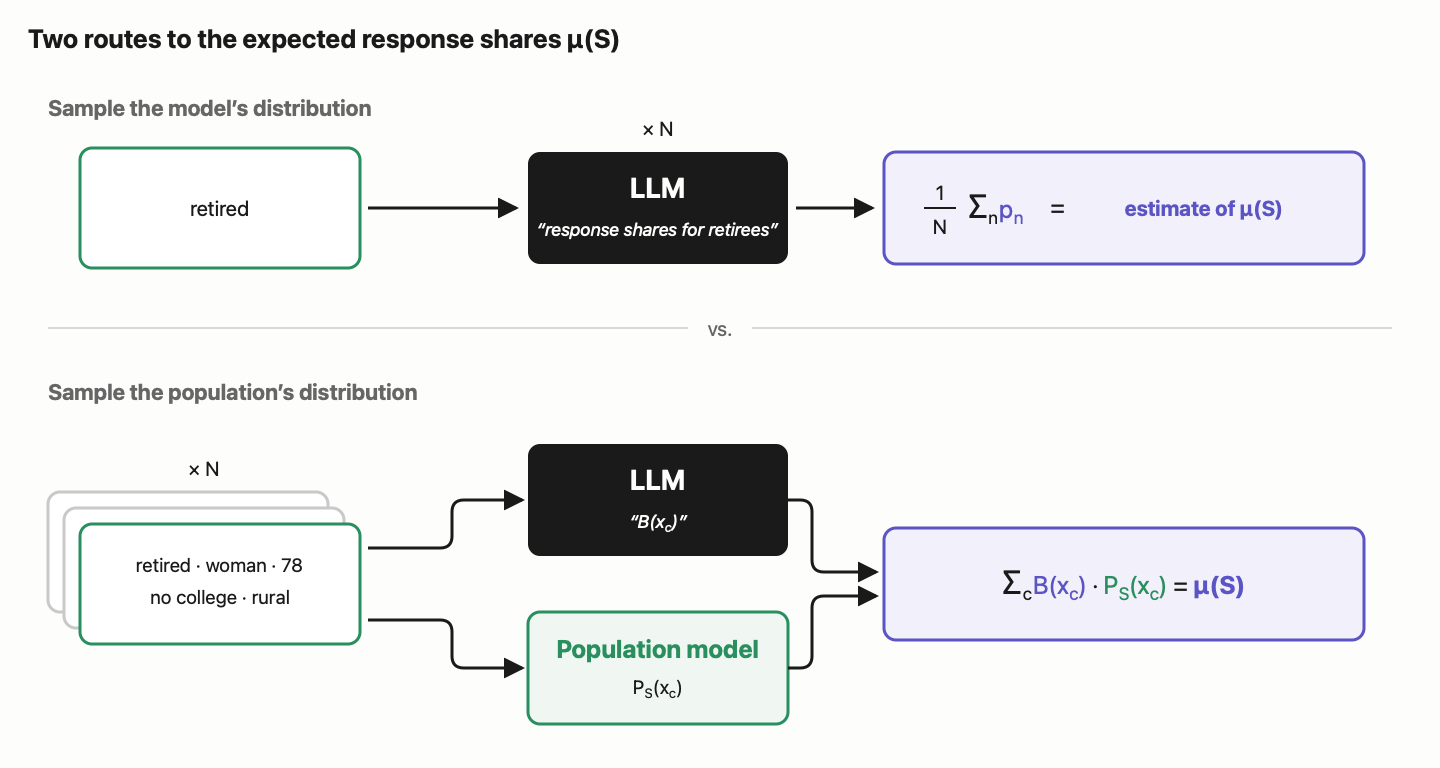
Both routes target the same estimate. The direct route hides the subgroup’s composition and the marginalization inside one model response, while the composed route obtains \(B(x)\) and \(P_{\mathcal S}(x)\) separately and takes their weighted sum outside the model.
To make the composed route reusable, we need to query the LLM once and turn its behavioral responses into a model we can evaluate offline.
3. Distilling a Behavior Model
For a given question, we want a behavioral model mapping an individual’s attributes \(x = (a_1, a_2, a_3, \dots)\) to a probability distribution over mutually exclusive response choices, where \(a_j\) is the individual’s level of attribute \(j\). For this post, we choose a simple, interpretable structure which is standard for modeling how individuals decide among discrete options.
3.1 Additive effect scores
We treat person-level attributes as categorical, or discretize them into categorical levels. For each response \(r\), we assign a baseline score \(b_r\) and a contribution \(w_r(a_j)\) from the persona’s level of each attribute \(j\). We then approximate the persona’s total score for response \(r\) as their sum:
\[s_r(x) = b_r + \sum_j w_r(a_j).\]This main-effects approximation replaces a separate parameter for every possible persona with a finite collection of attribute-level effects. Section 4 tests what we lose by omitting interactions.
The scores are not themselves probabilities. Normalizing their exponentials over the response options gives the response field:
\[B_r(x) = \frac{\exp s_r(x)}{\sum_{r'} \exp s_{r'}(x)}.\]We use \(B(x)\) for the full distribution over responses, with \(B_r(x)\) denoting the probability assigned to response \(r\).
3.2 Effects table and multi-hot encoding
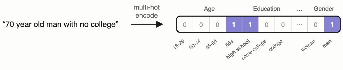
Because the attributes are categorical, there is a finite number of levels across all attributes, which we call \(D\). We flatten those levels into a single list and write the multi-hot encoding of persona \(x\) as \(\mathbf{x} \in \{0,1\}^D\), with one active entry for the persona’s level of each attribute.
With \(R\) possible response options, the attribute-level contributions can be stored in a lookup table \(W=[w_{rd}]\) with dimensions \(R \times D\). Its rows are response options, its columns are attribute levels, and each entry \(w_{rd}\) holds the contribution for response \(r\) and flattened attribute-level column \(d\). The table has the same response-by-attribute structure as a contingency table, but its cells contain log-linear effect scores rather than counts.
After flattening, the same score sum for a single response can be written as
\[s_r(x) = b_r + \sum_d w_{rd}\,\mathbf{x}_d.\]Multiplying the full multi-hot persona vector by the table performs that sum for every response at once:
\[s(x) = b + \mathbf{x}W^\top.\]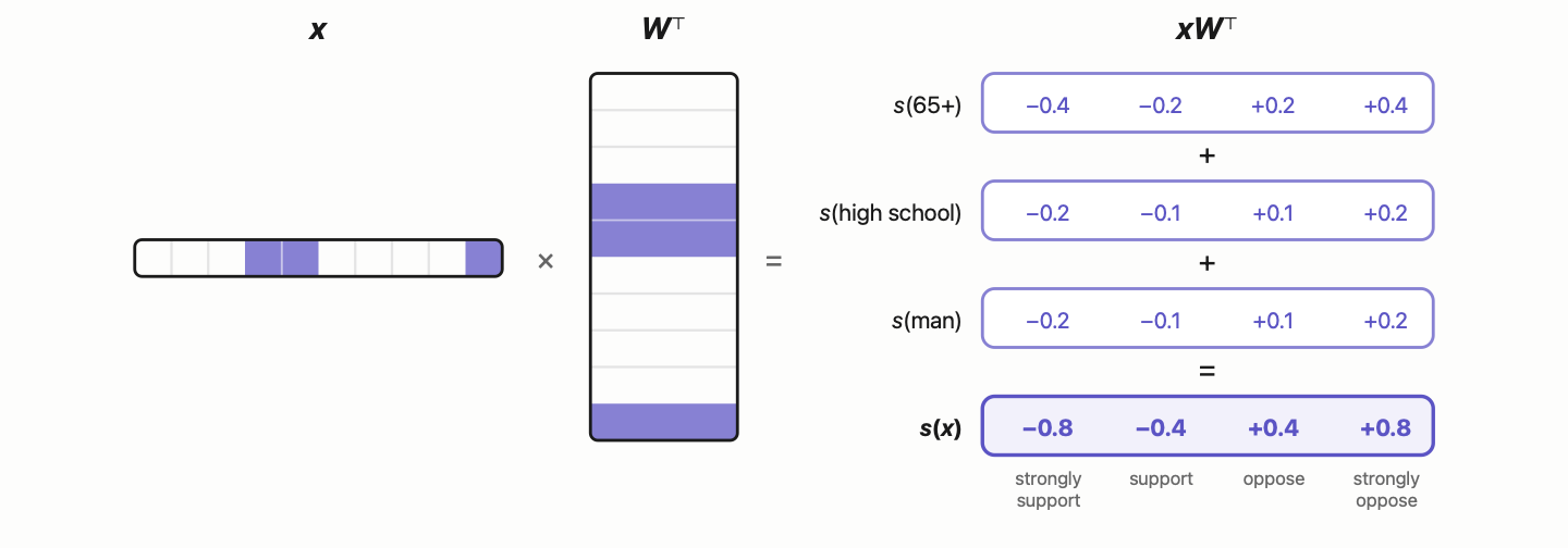
3.3 Learning the effects
Combining the table with the normalization above gives
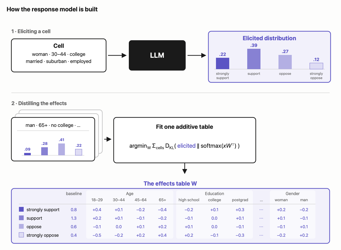
\[B(x) = \operatorname{softmax}(\mathbf{x}W^\top + b).\]This form is multinomial logistic regression. We treat the LLM as an oracle teacher \(\pi_{LLM}(\cdot \mid x)\) that returns a full probability distribution over response options for any given profile prompt. To fit our student policy \(B(x)\), we query the oracle across a training set of \(N\) persona states \(x^{(i)}\) and minimize the empirical forward KL divergence:
\[\pi^* = \arg\min_\pi \frac{1}{N} \sum_{i=1}^N \operatorname{KL}\big(\pi_{LLM}(x^{(i)}) \,\|\, \pi(x^{(i)})\big)\]Because the oracle returns complete soft distributions over all response categories rather than single discrete samples, minimizing forward KL is equivalent to minimizing soft-label cross-entropy. How many queried profile states the fit needs is the subject of Section 4.
3.4 One fit, any target subgroup
Once fitted, the same response model can be applied to any target subgroup defined by attributes in its schema. A subgroup \(\mathcal S\) identifies the set of complete persona cells consistent with its specified attributes. For women aged 65 and older, for example, age and gender are fixed while education, income, race, and the other modeled attributes vary across the compatible cells.
We poststratify by averaging the response model’s predictions over those cells, weighted by their prevalence within the subgroup:
\[\mu_r(\mathcal S) = \sum_{x \in \mathcal S} B_r(x)\,P(X{=}x \mid X \in \mathcal S).\]The behavior model \(B\) remains fixed, since changing the target subgroup changes only the population weights.
4. Evaluating the Elicitation Budget
Because we elicit a distribution over all responses for every persona, learning \(B(x)\) is a designed curve-fitting problem. We need enough well-placed reads to identify the effects and average over the parts of the oracle’s surface which are not perfectly additive.
4.1 The theoretical floor
For a main-effects model, the number of distinct persona cells needed to identify the design is
\[p = 1 + \sum_j (L_j - 1),\]where \(L_j\) is the number of levels of attribute \(j\). This minimum can be constructed from one reference cell and \(p-1\) additional cells which change one attribute at a time.
In our primary binary experiment, the schema contains 15 attributes and 74 levels, giving \(p=60\). Each elicitation supplies a distribution over every response option, so under a full-rank design and fixed identification constraints, these cells identify the response-specific effects in parallel. Additional cells then force the table toward the best additive description of the broader response surface rather than the particular reads in the minimum design.
4.2 The practical requirement
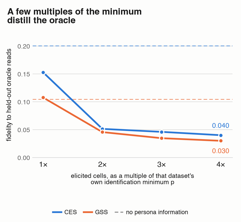
To test how many additional cells we needed, we fit tables using training sample counts from \(p\) to \(4p\) and scored each table against the LLM’s elicitations for held-out persona cells. Most of the improvement from adding training cells appeared by \(2p\), or 120 LLM elicitations in the primary experiment.
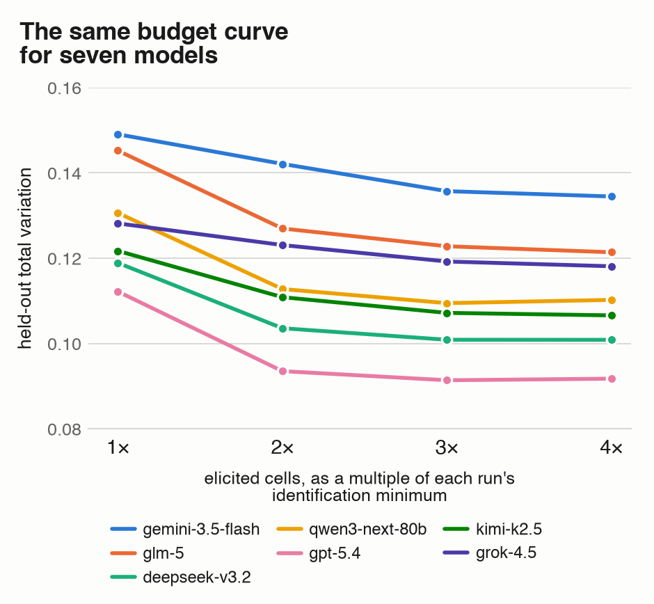
A companion evaluation repeated the budget curve on a second survey with multiclass response options and tables distilled from seven different LLMs. Although absolute performance varied across settings and source LLMs, the curves had remarkably similar shapes, with most of the attainable fidelity arriving at a relatively small elicitation budget.
4.3 The convergence gap
The held-out error nevertheless flattened above zero. Since the main-effects fit is convex, optimization was not the problem. Taking the full span from a persona-free guess to the oracle as 100%, the additive table closed about 80%, while better cell placement could recover another 2%, read noise accounted for 1%, and the limitations of the additive model accounted for the remaining 17%.

Pairwise interactions recovered about a sixth of the remaining gap, while higher-order terms bought essentially nothing further. We therefore retained the simpler main-effects model in the post’s other experiments.
5. The Oracle Is Not Ground Truth
While we refer to the LLM as our oracle, a high-fidelity distillation of an inaccurate model is still only as good as the model it copies.
We therefore distinguish fidelity and accuracy with two separate measures:
- Oracle fidelity measures how much distance the table closes between a persona-free baseline and the LLM’s held-out answers.
- Ground-truth accuracy measures how much of the progress from the same persona-free baseline to the best additive fit of held-out human data the distilled table achieves.
Both are normalized gap-closed measures in which zero represents the persona-free baseline, one represents the corresponding target, and higher values are better. The seven-model comparison below comes from the companion evaluation introduced in Section 4.2.
| model | oracle fidelity | ground-truth accuracy |
|---|---|---|
| gemini-3.5-flash | 0.530 | 0.511 |
| grok-4.5 | 0.595 | 0.489 |
| glm-5 | 0.597 | 0.484 |
| deepseek-v3.2 | 0.652 | 0.463 |
| qwen3-next-80b | 0.630 | 0.454 |
| gpt-5.4 | 0.660 | 0.435 |
| kimi-k2.5 | 0.556 | 0.422 |
Among these seven models, fidelity to the oracle did not predict accuracy against people. Gemini produced the least faithful distillation in the comparison, yet the most accurate one against ground truth. The table can copy its oracle well while inheriting the oracle’s systematic errors.
That leaves the more useful diagnostic question of whether the oracle is wrong about how groups differ from one another, or instead captures those differences while placing them on the wrong absolute scale.
6. Can the Student Surpass the Teacher?
Recall from Section 3 that our log-linear effects model is composed of a global baseline \(b\), shared by every group, and attribute-effect scores \(W\), which describe how groups deviate from that baseline. We can evaluate the two separately to diagnose whether our model’s errors reflect a misunderstanding of how attributes drive behavior, or a useful relative structure anchored to the wrong prior.
6.1 Scoring our scores
Returning to the primary binary experiment, we evaluate how well \(W\) captures the divergence between groups by measuring Spearman rank correlation between the model’s predictions and the ground-truth response rates. This gives us a proxy for the model’s relative structure, separately from the accuracy of its absolute predictions.
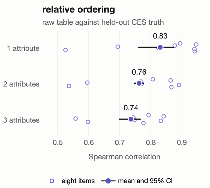
A Spearman correlation of 0.82 indicates strong agreement between the model’s ranking of groups and the ranking observed in the ground truth.
For the binary evaluation reported here, the predicted probability is monotone in the log odds between the two responses. Taking \(r_0\) as the reference response,
\[\log \frac{B_r(x)}{B_{r_0}(x)} = (b_r - b_{r_0}) + \sum_j \left[\,w_r(a_j) - w_{r_0}(a_j)\,\right] = \alpha_r + \sum_j \sum_{v \in \text{vals}(A_j) \setminus \{v_{j,0}\}} \beta_{j,v,r} \cdot \mathbf{1}[a_j = v]\]where \(\alpha_r = b_r - b_{r_0}\) represents the baseline log-odds intercept for response \(r\) and \(\beta_{j,v,r}\) are the identified attribute-effect contrasts relative to reference category levels \(v_{j,0}\).
The baseline contrast is constant across groups, so their ordering is determined entirely by the attribute effects in \(W\) (or \(\beta\)). The correlation therefore suggests that the model (and, by extension, the LLM from which it was distilled) has learned a substantial part of the relative geometry of the group-behavior space, narrowing the source of the remaining error.
6.2 A baseline diagnostic
While \(W\) determines how groups differ from one another, \(b\) determines the baseline from which those differences are measured. Having found that the model captures the relative ordering of groups well, we next ask whether its poor absolute predictions can be explained in part by an incorrect baseline.
To test this, we hold the learned attribute scores \(W\) fixed and optimize only a replacement baseline \(\tilde b\) against the held-out ground-truth data. This is a diagnostic rather than a deployable procedure because it uses the same cell-level human responses against which the model is evaluated.
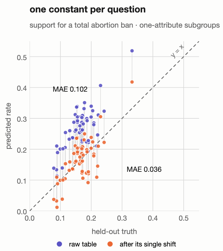
As the figure shows, replacing the original baseline with \(\tilde b\), while leaving every attribute score intact, reduces mean absolute error by up to 65% across the evaluated source models, and by an average of 31%. Because this adjustment is shared across groups, it improves the model’s absolute position without relearning the score differences encoded by \(W\). This suggests that a large part of the error lies in the overall distribution to which the group structure is anchored.
Here, the training targets were elicited from an LLM rather than sampled from a population. One plausible interpretation is that the LLM has systematic response-level preferences which cause it to overstate some answers and understate others, even while representing the differences between demographic groups reasonably well.
Re-estimating the baseline corrects a global shift but cannot address every distortion, including any tendency to overstate or understate differences between groups. The calibration below therefore addresses only the baseline error. Because the diagnostic also uses more outcome information than would be available in practice, we next ask whether an observable population topline can anchor the same response field.
7. Calibrate Once, Then Compose
Composing the raw response table over the global population distribution \(P_G(x)\) gives us the national response distribution implied by the model. Holding the learned attribute effects \(W\) fixed, we solve for a new baseline \(b^\star\) which shifts that implied distribution to match the observed topline \(T_G\):
\[\sum_x \operatorname{softmax}\!\left(\mathbf{x}W^\top + b^\star\right) P_G(x) = T_G.\]Whereas \(\tilde b\) uses cell-level human responses to diagnose the error, \(b^\star\) uses the topline as its only outcome information. Although the topline cannot answer any subgroup question by itself, it anchors every persona prediction produced by the same response field. Later subgroup estimates can then be obtained by composing the calibrated table with \(P_{\mathcal S}(x)\), with no further LLM calls.
For a fair comparison, we repeat the direct ask with the same topline supplied in its prompt, separating the value of the anchor from the value of explicit composition.
| estimator | no anchor | topline supplied |
|---|---|---|
| Direct group ask | 0.0449 | 0.0326 |
| Explicit composition | 0.0511 | 0.0239 |
| estimator | no anchor | topline supplied |
|---|---|---|
| Direct group ask | 0.0548 | 0.0414 |
| Explicit composition | 0.0702 | 0.0417 |
Mean absolute error, lower is better. Bold marks the better method within a column, and both anchored GSS values are bold because their difference is statistically indistinguishable.
Without an outcome anchor, the direct ask beats the raw composed table on both datasets, showing that distillation makes the response field reusable without making its absolute rates accurate. Supplying the topline improves both routes, after which explicit composition moves ahead of the anchored direct ask on CES and reaches parity with it on GSS.
Across these two evaluations, the consistent result is that the anchor turns the raw composed table from worse than direct asking into a competitive or better subgroup estimator. Whether explicit composition supplies additional accuracy beyond the anchored direct ask depends on the setting.
Because CES supplies one rate for a binary outcome while GSS supplies a distribution over several response options, the difference between their results should not be interpreted as a clean dataset or domain effect.
The LLM’s reusable contribution is the relative conditional structure encoded in \(W\), not a population of sampled respondents or a trustworthy absolute baseline. We distill that structure once into an offline parametric student, calibrate its baseline level with observed aggregate marginals, and evaluate it over an explicit population frame. Every subsequent subgroup query is then fast, deterministic arithmetic with zero marginal LLM calls.
In this post, we evaluated this conditional distillation on single survey outcomes, borrowing the demographic context \(X\) directly from observed human microdata.
In practice, however, complete joint microdata across dozens of interacting demographic, behavioral, and attitudinal attributes rarely exists. If we want to simulate realistic, coherent populations across complex multi-variable profiles, we cannot rely on external datasets to supply the full joint distribution. We must generate that joint distribution ourselves. In the next post, we show how to factorize the entire population joint into a sequence of the very same conditional models we just built, chaining them into an autoregressive Distilled-Conditional Bayesian Network (DisCo-BN) that generates rich, coherent synthetic populations with no compounding rollout drift.
Citation
Please cite this work as:
Eigen, Henry. "Use the LLM to Build Your Simulator, Not to Be Your Simulator". Heigen Thought (Aug 2026). https://henry-eigen.github.io/2026/08/03/build-your-simulator.html
Or use the BibTeX citation:
@article{eigen2026simulator,
  title = {Use the LLM to Build Your Simulator, Not to Be Your Simulator},
  author = {Eigen, Henry},
  journal = {henry-eigen.github.io},
  year = {2026},
  month = {August},
  url = "https://henry-eigen.github.io/2026/08/03/build-your-simulator.html"
}